In-depth Model Fitting

This notebook demonstrates how calibration models can be fitted with the helper function calibr8.fit_scipy.

from matplotlib import pyplot
import numpy
import pandas
import scipy.stats

import calibr8

Generating fake data

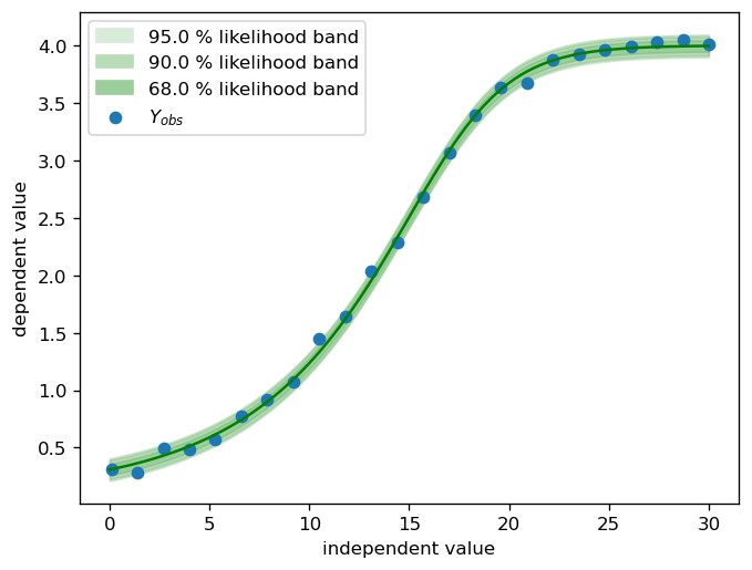
For the purpose of this notebook, a synthetic dataset is sufficient. The parameter vector of the ground truth model consists of two parts: \(\theta_µ\) and \(\theta_\sigma\).

θ_mu = (0.1, 4, 15, 0.3, 1) # 5 parameters of the asymmetric logistic
θ_scale = (0.05,)           # 1 parameter for constant scale
# concatenate all the parameter into one vector:
θ_true = θ_mu + θ_scale

# generate 24 calibration points with normal distributed noise
X = numpy.linspace(0.1, 30, 24)
Y = scipy.stats.norm.rvs(
    loc=calibr8.asymmetric_logistic(X, θ_mu),
    scale=calibr8.polynomial(X, θ_scale),
)

fig, ax = pyplot.subplots(dpi=120)

# plot the noise band of the ground truth
X_dense = numpy.linspace(0, 30, 100)
calibr8.plot_norm_band(
    ax,
    X_dense,
    mu=calibr8.asymmetric_logistic(X_dense, θ_mu),
    scale=calibr8.polynomial(X_dense, θ_scale),
)

ax.scatter(X, Y, label='$Y_{obs}$')

ax.set_xlabel('independent value')
ax.set_ylabel('dependent value')
ax.legend()
pyplot.show()

Setting up the model

Our data follows an asymmetric logistic ground truth with normal-distributed observation noise. The noise sigma is constant, so it can be modeled with a 0th-degree polynomial.

calibr8 already implements three commonly used model types that can be inherited and customized: + calibr8.BaseModelN implements likelihood and inference methods for normal-distributed noise models + calibr8.BasePolynomialModelN models mu and sigma as polynomials + calibr8.BaseAsymmetricLogisticModelN models mu as asymmetric logistic and sigma as polynomial The degress of the polynomials in BasePolynomialModelN and BaseAsymmetricLogisticModelN are user-defined.

class ToyAsymmetricModelV1(calibr8.BaseAsymmetricLogisticN):
    def __init__(self):
        super().__init__(
            independent_key='concentration_mM',
            dependent_key='absorbance_au',
            sigma_degree=0
        )

Fitting

Here we will not only fit the model, but also compare the two available fitting methods.

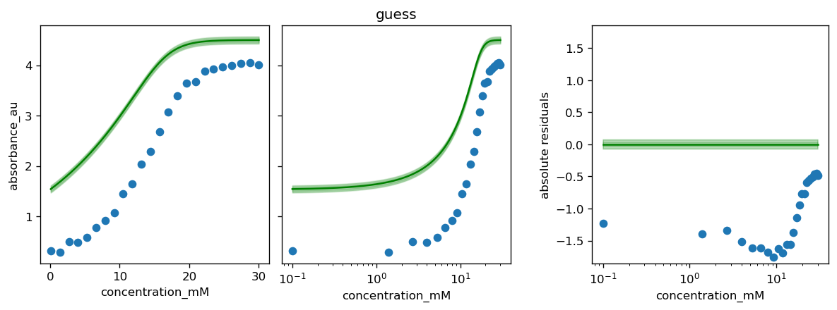
We begin by making initial guesses about \(\theta\) and the bounds of the parameter space.

The best way to make initial guesses is to scatter-plot the raw data and visually guess the limits, inflection point and slope. We already have a scatter plot above.

For more intuition about the parameters of the asymmetric logistic function, see the “Basic_GeneralizedLogistic” notebook that has an interactive plot where you can manipulate the parameters.

guess = [
    0,   # lower limit approximately at 0 ?
    4.5, # upper limit maybe around 4.5 ?
    12,  # inflection point maybe at arond 12 ?
    1/5, # approximate slope at inflection point
    2,   # asymmetry paramter: the inflection point is near the upper limit -> positive value
] + [
    numpy.ptp(Y)/100,  # constant noise at around 1 % of the amplitude
]

# bounds can be half-open, or closed:
# `fit_scipy` works best with half-open bounds for L_L and L_U
bounds_halfopen = [
    (-numpy.inf, 1),   # L_L
    (3.5, numpy.inf),  # L_U
    (10, 20),          # I_x
    (1/20, 1),         # S
    (-3, 3),           # c
] + [
    (0.01, 0.5), # min/max for scale
]

We’ll collect not only the fit results, but also the guess and ground truth in a DataFrame:

model = ToyAsymmetricModelV1()

df_results = pandas.DataFrame(columns=['method', 'θ']).set_index('method')
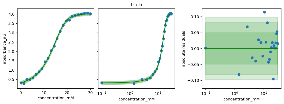
df_results.loc['truth', 'θ'] = θ_true
df_results.loc['guess', 'θ'] = guess
df_results

	θ
method
truth	(0.1, 4, 15, 0.3, 1, 0.05)
guess	[0, 4.5, 12, 0.2, 2, 0.037627665408536896]

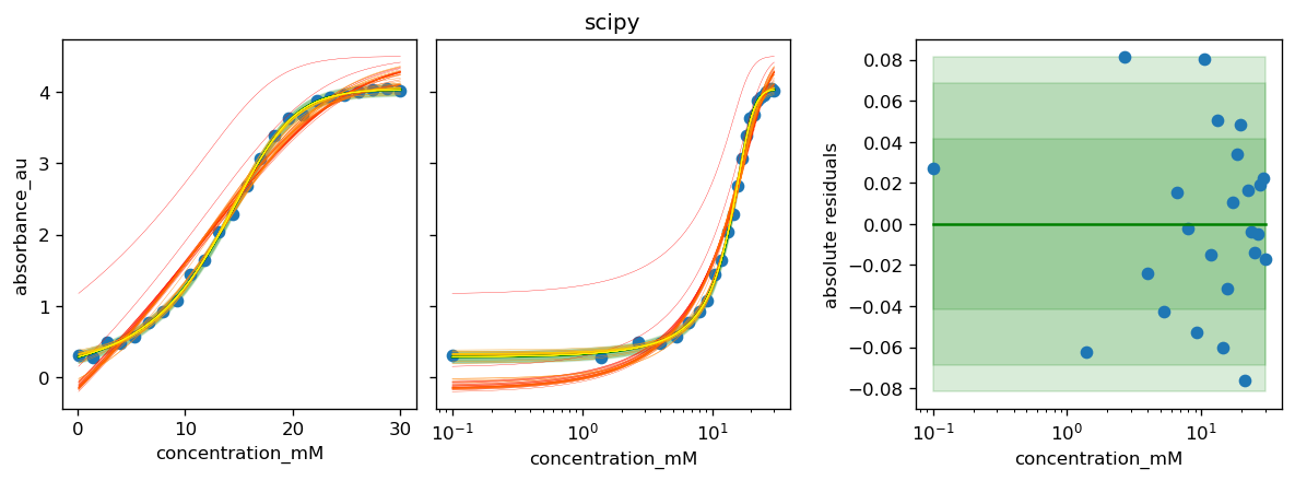
The fitting helper methods return a tuple of the best found θ and a list of historic parameter sets during the optimization.

The history will later be used to visualize the optimization over time.

df_results.loc['scipy', 'θ'], history_scipy = calibr8.fit_scipy(
    model,
    independent=X, dependent=Y,
    theta_guess=guess,
    theta_bounds=bounds_halfopen
)

Now that parameter vectors were found, we can add a “loglikelihood” column to compare the results:

df_results['loglikelihood'] = [
    model.loglikelihood(x=X, y=Y, theta=θ)
    for θ in df_results['θ']
]
df_results

	θ	loglikelihood
method
truth	(0.1, 4, 15, 0.3, 1, 0.05)	39.048817
guess	[0, 4.5, 12, 0.2, 2, 0.037627665408536896]	-12718.564797
scipy	[0.03816243158544993, 4.036333518903234, 14.84...	42.226240

def plot_fit_history(axs, model, history):
    X = model.cal_independent
    for i, x in enumerate(history):
        x_dense = numpy.exp(numpy.linspace(numpy.log(min(X)), numpy.log(max(X)), 1000))
        mu, _ = model.predict_dependent(x_dense, theta=x)
        axs[0].plot(x_dense, mu, color=pyplot.cm.autumn(i / len(history)), linewidth=0.2)
        axs[1].plot(x_dense, mu, color=pyplot.cm.autumn(i / len(history)), linewidth=0.2)
    return


for method, history in zip(df_results.index, [None, None, history_scipy]):
    # the plot_model method uses model.theta_fitted
    # here we override it with the parameter set found by a certain method
    model.theta_fitted = df_results.loc[method, 'θ']

    fig, axs = calibr8.plot_model(model)
    if history is not None:
        plot_fit_history(axs, model, history)
    axs[1].set_title(method)
    fig.tight_layout()
    pyplot.show()

C:\Users\osthege\AppData\Local\Temp\ipykernel_24424\1783795081.py:20: UserWarning: This figure includes Axes that are not compatible with tight_layout, so results might be incorrect.
  fig.tight_layout()

%load_ext watermark
%watermark -n -u -v -iv -w

The watermark extension is already loaded. To reload it, use:
  %reload_ext watermark
Last updated: Tue Dec 13 2022

Python implementation: CPython
Python version       : 3.9.15
IPython version      : 8.7.0

sys       : 3.9.15 (main, Nov 24 2022, 14:39:17) [MSC v.1916 64 bit (AMD64)]
pandas    : 1.4.3
scipy     : 1.9.0
numpy     : 1.23.1
matplotlib: 3.5.3
calibr8   : 6.6.1

Watermark: 2.3.1