import ipywidgets
import numpy
from matplotlib import pyplot

import calibr8

The Generalized Logistic Function

Real-world calibration curves rarely follow linear dose/response relationships, but often exhibit lower & upper saturations. These relationships can be described with S-shaped functions. The logistic function (the sigmoid curve is a special case of it) is often well suited for real-world calibration curves.

Several different flavors of S-shaped curves are available:

• sigmoid (1 parameter: variable slope)

• logistic (3 parameters: variable upper limit, variable x-value of the inflection point, variable slope)

• generalized logistic (5 parameters: variable limits, variable inflection point, variable slope, variable symmetry)

Here, we’re going to use the generalized logistic, because it is most useful. However, we use a different parametrization that is derived in the notebook Background_AsymmetricLogistic.

\[f(x)= L_L \cdot (L_U - L_L) \cdot (e^{(\frac{S}{L_U - L_L} (I_{x} - x) + c (e^{c} + 1)^{-(e^{c} + 1) e^{- c}}) (e^{c} + 1)^{(e^{c} + 1) e^{- c}}} + 1)^{- e^{- c}}\]

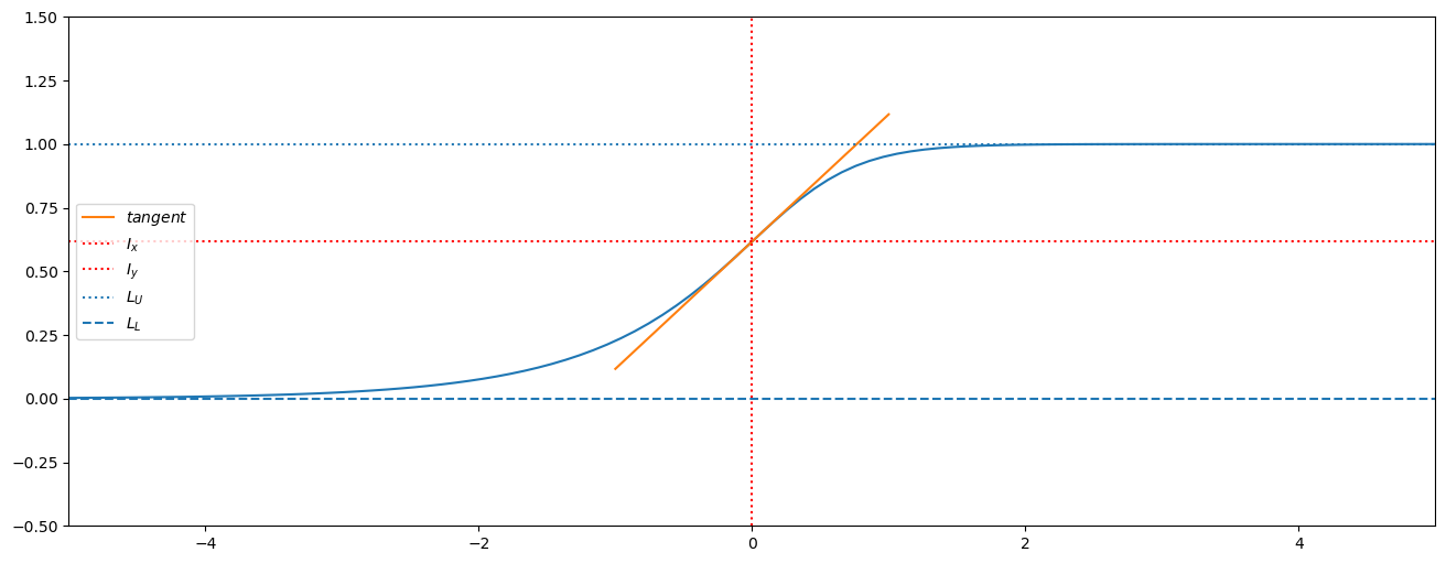
The following table shows the bounds & interpretation of its 5 paramters:

parameter	interpretation
\(L_L \in \mathcal{R}\)	lower asymptote
\(L_U \in \mathcal{R}\)	upper asymptote
\(I_x \in \mathcal{R}\)	x-value of the inflection point
\(S \in \mathcal{R}\)	slope at the inflection point I_x
\(c \in \mathcal{R}\)	moves the inflection point closer to L_L (c < 0) or closer to L_U (0 < c).

Example

Let’s say we have an assay with noticeable lower- and upper satuation limits, as well as some asymmetry.

To visualize the meaning of the parameters, we can draw an interactive plot of the calibr8.asymmetric_logistic function:

help(calibr8.asymmetric_logistic)

Help on function asymmetric_logistic in module calibr8.core:

asymmetric_logistic(x, theta)
    5-parameter asymmetric logistic model.

    Parameters
    ----------
    x : array-like
        independent variable
    theta : array-like
        parameters of the logistic model
            L_L: lower asymptote
            L_U: upper asymptote
            I_x: x-value at inflection point
            S: slope at the inflection point
            c: symmetry parameter (0 is symmetric)

    Returns
    -------
    y : array-like
        dependent variable

def tangent(I_x, I_y, S):
    """Get x,y to plot a line with slope S around the coordinate <I_x,I_y>."""
    x = numpy.linspace(I_x - 1, I_x + 1, 2)
    y = -S * I_x + I_y + S * x
    return x, y


def plot_logistic(L_L=0, L_U=1, I_x=0.0, S=0.5, c=1.0):
    theta = (L_L, L_U, I_x, S, c)
    X_MIN, X_MAX = -5, 5
    X = numpy.linspace(-5, 5, 100)

    # get key properties to visualize
    I_y = calibr8.asymmetric_logistic(I_x, theta)

    fig, ax = pyplot.subplots(figsize=(16, 6))
    ax.plot(X, calibr8.asymmetric_logistic(X, theta))
    ax.plot(*tangent(I_x, I_y, S), label="$tangent$")

    ax.axvline(I_x, linestyle=":", color="red", label="$I_x$")
    ax.axhline(I_y, linestyle=":", color="red", label="$I_y$")
    ax.axhline(L_U, linestyle=":", label="$L_U$")
    ax.axhline(L_L, linestyle="--", label="$L_L$")

    ax.set_xlim(X_MIN, X_MAX)
    ax.set_ylim(L_L - 0.5, L_U + 0.5)
    ax.legend(loc="center left")
    pyplot.show()


plot_logistic()
ipywidgets.interact(
    plot_logistic, L_L=(-5.0, 0), L_U=(0.0, 5), I_x=(-5.0, 5), S=(-2.0, 3), c=(-2.0, 2)
);

Summary

• The generalized logistic function can describe relationships with lower & upper satuation

• Even in cases of “good linear relationships”, the GLF is applicable

• The original parameterization is not very intuitive, but was reparameterized such that 4 of 5 parameters are interpretable

%load_ext watermark
%watermark -n -u -v -iv -w

Last updated: Wed, 15 Apr 2026

Python implementation: CPython
Python version       : 3.13.12
IPython version      : 9.11.0

calibr8   : 7.2.0
ipywidgets: 8.1.8
matplotlib: 3.10.8
numpy     : 2.4.2
platform  : 1.0.8

Watermark: 2.6.0