Numeric posterior of the independent variable

In this notebook, we demonstrate the use of infer_independent and predict_independent. Given observations \(Y_{obs}\) made at the same corresponding independent variable (e.g. several slightly different measurements of the same glucose concentration), infer_independent will return a probability distribution taking all observations into account. predict_independent will only return the median of a distribution under the assumption that this was the only observation. For a uniform prior, the posterior inferred by MCMC yields the same result as a numerically integrated likelihood function, which is demonstrated at the end of the notebook.

import ipywidgets
import numpy
import pymc as pm
import scipy.stats
from matplotlib import pyplot

import calibr8

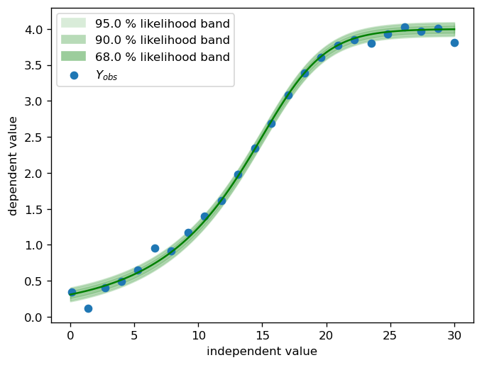
Synthetic groundtruth

θ_true = (0.1, 4, 15, 0.3, 1)
σ_true = 0.05
df_true = 1.5
X = numpy.linspace(0.1, 30, 24)
X_dense = numpy.linspace(0, 30, 100)
Y = calibr8.asymmetric_logistic(X, θ_true)
numpy.random.seed(230620)
Y = scipy.stats.t.rvs(loc=Y, scale=σ_true, df=df_true)

fig, ax = pyplot.subplots(dpi=120)

calibr8.plot_norm_band(
    ax, X_dense, calibr8.asymmetric_logistic(X_dense, θ_true), σ_true
)

ax.scatter(X, Y, label="$Y_{obs}$")

ax.set_xlabel("independent value")
ax.set_ylabel("dependent value")
ax.legend()
pyplot.show()

Model definition

class AsymmetricTModelV1(calibr8.BaseAsymmetricLogisticT):
    def __init__(self):
        super().__init__(
            independent_key="independent", dependent_key="dependent", scale_degree=0
        )

Model fit

model = AsymmetricTModelV1()
calibr8.fit_scipy(
    model,
    independent=X,
    dependent=Y,
    theta_guess=[
        0,  # lower limit approximately at 0 ?
        4.5,  # upper limit maybe around 4.5 ?
        12,  # inflection point maybe at arond 12 ?
        1 / 5,  # approximate slope at inflection point
        2,  # asymmetry paramter: the inflection point is near the upper limit -> positive value
    ]
    + [0.01, 5],
    theta_bounds=[
        (-numpy.inf, 1),  # L_L
        (3.5, numpy.inf),  # L_U
        (10, 20),  # I_x
        (1 / 20, 1),  # S
        (-3, 3),  # c
    ]
    + [(0.01, 0.5), (0.5, 50)],
)

fig, axs = calibr8.plot_model(model)
pyplot.show()
print(
    f"The following estimations were made for {model.theta_names}: {model.theta_fitted}"
)

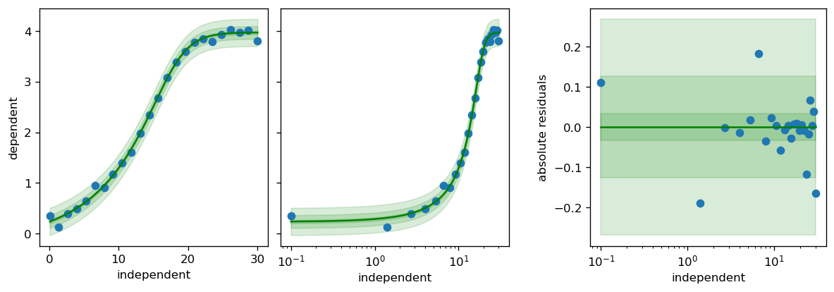
The following estimations were made for ('L_L', 'L_U', 'I_x', 'S', 'c', 'scale_0', 'df'): (np.float64(-0.16185161895575242), np.float64(3.974966313239348), np.float64(15.262603589530178), np.float64(0.28658757430416437), np.float64(1.3554343266920206), np.float64(0.01744906898419064), np.float64(0.9251011065918714))

Visualization

def plot(y_obs=0.5, a=0, b=30, steps=1000, ci_prob=0.95):
    y_obs = numpy.atleast_1d(y_obs)
    fig, ax = pyplot.subplots(dpi=120)

    posterior = model.infer_independent(
        y_obs, lower=a, upper=b, steps=steps, ci_prob=ci_prob
    )
    ax.plot(posterior.hdi_x, posterior.hdi_pdf, color="b")

    # Plot the individual predictions from predict_independent for comparison
    for yo in y_obs:
        ax.axvline(model.predict_independent(yo), linestyle="--", color="b", alpha=0.3)
    ax.plot(
        [], linestyle="--", label="predict_independent", color="b", alpha=0.3
    )  # to get only one legend

    # For multiple observations of the same independent variable,
    # the median of the posterior will differ from the two predict_independent results
    ax.annotate(
        "median",
        xy=(posterior.median, 0),
        xytext=(posterior.median, numpy.max(posterior.hdi_pdf) * 0.2),
        xycoords="data",
        arrowprops=dict(facecolor="b", edgecolor="b", shrink=0.05),
        horizontalalignment="right",
        verticalalignment="top",
        ha="center",
    )

    ax.legend()
    ax.set_xlabel("independent variable")
    ax.set_ylabel(r"$p(x\ |\ \vec{y}_{obs})$")
    ax.set_ylim(0)
    return fig, ax

Plot for one observation, where predict_independent is similar to the median

def iplot(y_obs=0.5, a=0, b=30, steps=1000, ci_prob=0.95):
    plot(y_obs, a, b, steps, ci_prob)
    pyplot.show()


ipywidgets.interact(
    iplot,
    y_obs=θ_true[0:2],
    a=ipywidgets.fixed(0),
    b=ipywidgets.fixed(30),
    steps=ipywidgets.fixed(1000),
    percentiles=ipywidgets.fixed((0.025, 0.975)),
);

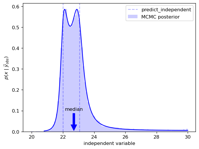
Comparison with MCMC for two observations

y_obs = numpy.array([3.85, 3.9])
a = 0
b = 30

theta = model.theta_fitted
with pm.Model():
    prior = pm.Uniform(model.independent_key, lower=a, upper=b)
    mu, scale, df = model.predict_dependent(prior, theta=theta)
    pm.StudentT("likelihood", nu=df, mu=mu, sigma=scale, observed=y_obs)
    idata = pm.sample(10_000, cores=4)

C:\Users\osthege\AppData\Local\miniforge3\envs\dibecs_9.2.1\Lib\site-packages\threadpoolctl.py:1226: RuntimeWarning:
Found Intel OpenMP ('libiomp') and LLVM OpenMP ('libomp') loaded at
the same time. Both libraries are known to be incompatible and this
can cause random crashes or deadlocks on Linux when loaded in the
same Python program.
Using threadpoolctl may cause crashes or deadlocks. For more
information and possible workarounds, please see
    https://github.com/joblib/threadpoolctl/blob/master/multiple_openmp.md

  warnings.warn(msg, RuntimeWarning)
Initializing NUTS using jitter+adapt_diag...
Multiprocess sampling (4 chains in 4 jobs)
NUTS: [independent]

Sampling 4 chains for 1_000 tune and 10_000 draw iterations (4_000 + 40_000 draws total) took 32 seconds.

Here we can see how the median differs from predict_independent results

fig, ax = plot(y_obs=y_obs, ci_prob=0.999)
ax.hist(
    idata.posterior["independent"].stack(sample=("chain", "draw")).values.T,
    density=True,
    bins=100,
    color="b",
    alpha=0.2,
    label="MCMC posterior",
)
ax.legend()
pyplot.show()

%load_ext watermark
%watermark -n -u -v -iv -w

Last updated: Wed, 15 Apr 2026

Python implementation: CPython
Python version       : 3.13.12
IPython version      : 9.11.0

calibr8   : 7.2.0
ipywidgets: 8.1.8
matplotlib: 3.10.8
numpy     : 2.4.2
platform  : 1.0.8
pymc      : 5.28.1
scipy     : 1.17.1

Watermark: 2.6.0