Fitting a Linear Model

This notebook demonstrates how to build the most basic model with calibr8.

We begin with importing the relevant packages:

import numpy
from matplotlib import pyplot

import calibr8

Inspecting the calibration data points

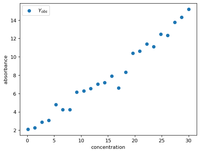
At the beginning of almost every data analysis it is always a good idea to take a brief look at the data.

For the purpose of this notebook, the dataset is randomly generated.

# generate 24 calibration points with t-distributed noise
numpy.random.seed(666)
N = 24
X = numpy.linspace(0.1, 30, N)
Y = 1.7 + 0.43 * X + 0.5 * numpy.random.standard_t(df=3, size=N)

fig, ax = pyplot.subplots(dpi=120)
ax.scatter(X, Y, label="$Y_{obs}$")
ax.set_xlabel("concentration")
ax.set_ylabel("absorbance")
ax.legend()
pyplot.show()

Setting up the model

A linear function is the 2nd-simplest version of a polynomial. (The simplest being a 0th-order polynomial–a constant–but that”s not very helpful here.)

To create a linear model, we can use the calibr8.BasePolynomialModelT and specify a mu_degree=1.

The Base...ModelT uses a Student-t distribution, which is robust against outliers and has some numerical advantages for modeling.

class ToyLinearModelV1(calibr8.BasePolynomialModelT):
    def __init__(self):
        super().__init__(
            independent_key="concentration",
            dependent_key="absorbance",
            mu_degree=1,
            scale_degree=0,
        )


model = ToyLinearModelV1()

Fitting the model to data

A calibr8.CalibrationModel is typically fitted by optimization using one of the helper functions from the calibr8.optimization module.

The fit_scipy helper function works for about 90 % of the cases. If you have trouble finding a good fit for your model, you can try to make a better initial guess of the parameters and specify tighter bounds. For more tips on model fitting, see the “In-depth Model Fitting” example.

# the helper function returns:
# + the optimized model parameter vector `theta_fit`
# + the history of parameter vectors tested in the optimization
# It also assignes some relevant variables to the `model`.
theta_fit, history = calibr8.fit_scipy(
    model=model,
    independent=X,
    dependent=Y,
    theta_guess=[1, 0.5, 1, 1],
    theta_bounds=[
        (-2, 5),
        (0, 2),
        (0.01, 5),
        (1, 50),
    ],
)

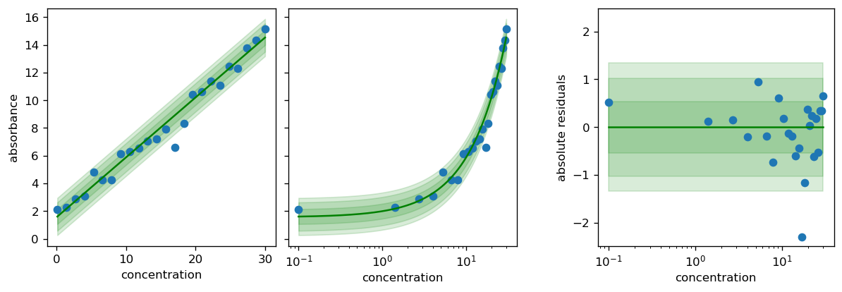
After the fit_scipy function ran without warnings, we can use the calibr8.plot_model function to inspect the model fit.

# the function returns the matplotlib Figure and Axes, so you can do more with it.
fig, axs = calibr8.plot_model(model)
pyplot.show()

Alternatively, you can use the fit_scipy_global helper function which does not require an initial guess and can handle wider bounds, but entails a longer computation time.

The procedure does not differ much when using global optmization.

theta_fit, history = calibr8.fit_scipy_global(
    model=model,
    independent=X,
    dependent=Y,
    theta_bounds=[
        (-20, 20),
        (0, 20),
        (0, 20),
        (1, 100),
    ],
)

C:\Users\osthege\AppData\Local\miniforge3\envs\dibecs_9.2.1\Lib\site-packages\scipy\stats\_distn_infrastructure.py:2117: RuntimeWarning: divide by zero encountered in divide
  x = np.asarray((x - loc)/scale, dtype=dtyp)

# the function returns the matplotlib Figure and Axes, so you can do more with it.
fig, axs = calibr8.plot_model(model)
pyplot.show()

Using the fitted model

One common use case for such a calibration model is the inference of a dependent variable (concentration) from observations (absorbances).

All calibr8.CalibrationModels have a .infer_independent() method that numerically does this for you.

result = model.infer_independent(
    # we must pass one or more observations, and a lower/upper bound of plausible concentration
    y=[5.9, 6.0],
    lower=0,
    upper=30,
    ci_prob=0.9,
)
print(result)

<class 'calibr8.core.ContinuousUnivariateInference'>
    ETI (90.0 %): [8.8097, 11.4909] Δ=2.6812
    HDI (90.0 %): [8.8097, 11.4909] Δ=2.6812

The returned object is a calibr8.NumericPosterior with useful properties such as the median, or the hdi_lower and hdi_upper.

print(f"The median of the posterior is {result.median:.1f}")
print(
    f"With {result.hdi_prob * 100:.0f} % probabilty, "
    f"the concentration is between {result.hdi_lower:.1f} and {result.hdi_upper:.1f}."
)

The median of the posterior is 10.2
With 90 % probabilty, the concentration is between 8.8 and 11.5.

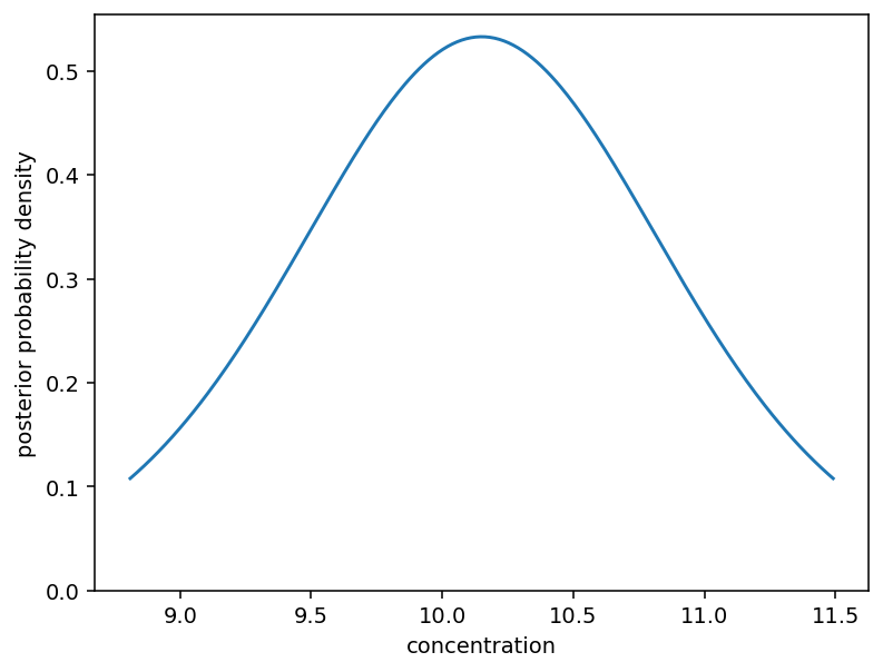
We can plot the posterior density from the .eti_x and .eti_pdf properties:

fig, ax = pyplot.subplots(dpi=140)
ax.plot(
    result.eti_x,
    result.eti_pdf,
)
ax.set_ylim(0)
ax.set_ylabel("posterior probability density")
ax.set_xlabel("concentration")
pyplot.show()

For more details on the .infer_independent() method, see the “Numeric Independent Posterior” example.

%load_ext watermark
%watermark -n -u -v -iv -w

Last updated: Wed, 15 Apr 2026

Python implementation: CPython
Python version       : 3.13.12
IPython version      : 9.11.0

calibr8   : 7.2.0
matplotlib: 3.10.8
numpy     : 2.4.2
platform  : 1.0.8

Watermark: 2.6.0