import numpy
from matplotlib import pyplot

import calibr8

WARNING (theano.tensor.blas): Using NumPy C-API based implementation for BLAS functions.

The Exponential Model

The exponential function is a rather simple formula that can be applied to quite a number of real-world problems. This example demonstrates how the calibr8.exponential model can describe four commonly seen trends in real world data.

It is available through base models such as calibr8.BaseExponentialModelN and calibr8.BaseExponentialModelT, but this example won’t go into detail with these and just look at the underlying calibr8.exponential function.

A picture says more than a thousand words, so before the details let’s see how it looks like:

B = 4
x = numpy.linspace(-B, B)

fig, axs = pyplot.subplots(ncols=2, nrows=2, figsize=(8, 8), dpi=150, sharex=True, sharey=True)

for ax, theta in zip(axs.flatten(), [
    (1, 2, 0.5),
    (1, 2, -0.5),
    (1, -1, 0.5),
    (1, -1, -0.5),
]):
    ax.axhline(0, color="black", lw=0.5)
    ax.axvline(0, color="black", lw=0.5)
    ax.plot(x, calibr8.exponential(x, theta))
    I, L, k = theta
    ax.axhline(L, ls="--", lw=0.5)
    ax.annotate(
        f"Limit=${L}$",
        xy=(0, L), xytext=(1, L),
        va="center",
        arrowprops=dict(arrowstyle="-|>", color="black")
    )
    ax.annotate(
        f"Intercept=${I}$",
        xy=(0, I), xytext=(1, I),
        va="center",
        arrowprops=dict(arrowstyle="-|>", color="black")
    )
    ax.text(s=f"k=${k}$", x=0.1, y=3)
    ax.set(
        ylim=(-B, B),
        xlim=(-B, B),
    )
fig.tight_layout()
pyplot.show()

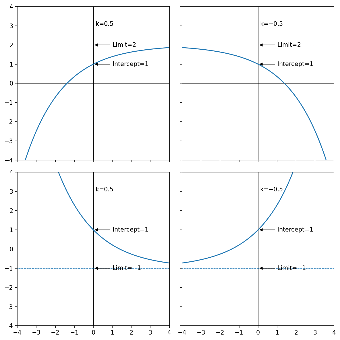
As you can see from the code and figure above, all flavors have the shape of a simple e-function, but it’s shifted, scaled and flipped around depending on: * Is the y-axis intercept I above, or below the asymptotic limit L? * Is the rate parameter k positive or negative?

We can have exactly four combinations of answers to these two or questions, that’s why we got four shapes.

The calibr8.exponential model is implemented as…

\[I + (L-I) \cdot (1-e^{-k \cdot x})\]

…because this way, the most common shape (approaching a limit from below) is obtained from all-positive parameters.

But as we saw above, each paramter has a real-valued support:

parameter	interpretation
\(I \in \mathcal{R}\)	y-axis intercept
\(L \in \mathcal{R}\)	asymptotic limit
\(k \in \mathcal{R}\)	exponential rate parameter

%load_ext watermark
%watermark -n -u -v -iv -w

Last updated: Wed Feb 23 2022

Python implementation: CPython
Python version       : 3.8.12
IPython version      : 7.31.0

matplotlib: 3.5.1
sys       : 3.8.12 | packaged by conda-forge | (default, Oct 12 2021, 21:22:46) [MSC v.1916 64 bit (AMD64)]
calibr8   : 6.4.0
numpy     : 1.20.3

Watermark: 2.3.0